The Math of Split Testing Part 2: Chance of Being Better

tl;dr

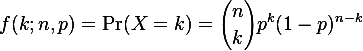
Split tests are a powerful way to determine if a new design has outperformed an old design. Here, we present the math necessary to empirically state the chance that a new design (branch B) is better than an old design (branch A). We walk through the problem with numerical simulations and present an approximate formula to easily determine the winner of an A/B test.

Split testing is the preferred way to collect data for fact based decision making. Longitudinal studies are subject to underlying market trends and are not well suited for conversion rate experiments. If, for example, you roll out a new version of your website in April and notice a decrease in conversion rate, you may be tempted to say that your new website design is a failure. But maybe April was just a bad month. If instead you had set up a split test for your new design, you could eliminate this concern. While overall conversions may have fallen in April, it could easily be the case that the results of a split test measurement would have shown the new website design performed 20% better than original design, with 95% chance that the new design is better than the original.

In this post, we’ll introduce the math necessary to declare branch A or branch B the winner of the split test. While the math in this post is self-contained, the origins of our analysis come from statistical sampling uncertainty, which we addressed in detail in Part 1: Statistical Sampling Uncertainty. Here, we’ll assume familiarity with statistical sampling uncertainty and begin our analysis by examining the binomial mass function.

The binomial probability mass function can be viewed in two complementary ways. The first way to view the probability mass function is to answer the question “If we flip a fair coin (p = 0.5) 100 times (n = 100), how likely is it that the coin lands on heads exactly 40 times (k = 40)”. Then you could ask how likely it was that it landed on heads exactly 41 times. Then 42 times. And so on. This would give you a nice plot of the probability of obtaining a variable number of heads for a fair coin after 100 flips. This is the sort of analysis we conducted in Part 1.

However, the binomial probability mass function can also be viewed as a variable of p. Looking at it this way answers the question “When we performed an experiment where we flipped a coin of unknown bias 100 times (n = 100). The result was that the coin landed on heads 40 times (k = 40). What is the probability that the coin was fairly biased (p = 0.5)?” Then ask the question how likely is is that the coin is weighted slightly towards heads, say a 0.51 bias towards heads. Then 0.52, etc.. Or maybe it was biased towards tails (0.49 heads bias). Collecting all of these results gives the following plot of the probability of a coin’s bias towards heads, given that we observed 40 heads in 100 flips.

The shape of the curve Poissonian, but the distribution tends toward Gaussian by the central limit theorem. Since the distribution is nearly Gaussian, it is often approximated to be Gaussian, with the rule of thumb that there should be at least 30 samples and an appropriate number of conversions, np > 5 and n(1-p) > 5. At the moment we need not concern ourselves with the exact shape of the distribution, we’ll just use the exact one generated from our computer simulation. However, we’d like to note that since we’re analyzing a measurement with only 100 samples, the distribution is quite wide with probable values of true coin bias falling between 0.3 and 0.5.

In Part 1 we discussed how to report a confidence interval for a single experiment like the one we just described. Now, we want to analyze the results of a split test, comprised of and two concurrently measured branches. For concreteness, let’s assume that we are split testing a new website design (branch B) against our old design (branch A).

Let’s say that we’re hoping our new design will be a home run so we only let the experiment run for a day. After collecting data on each branch for one day we end up with 45 conversions out of 100 visitors for our old design and 50 conversions out of 100 visitors for our new design. What’s the chance that our new design better than our old one?

Our new design (branch B) appears that it is better, after all it is > 10% better than branch A. But just like before, each of the branches is going to be subject to statistical sampling uncertainty. In order to determine if branch B has beaten branch A, we’re going to have to do some additional analysis. First, we’ll calculate the probability of true coin head bias for each branch using the binomial probability mass function. It looks like this:

To generate the plot, the probability was calculated for the original design (branch A), shown in blue, by fixing n at 100 samples and k at the observed value of 45 heads. We then calculated the probability of true coin bias by varying p. The same process was then repeated for our new design (branch B), shown in red, but with the appropriate value of k = 50 heads.

We can see from the plot that each distribution is rather wide and there is a good degree of overlap between them. The fact that each distribution is rather wide comes from the small sample size used to form the distribution. The separation between the center of each distribution is just the difference in observed conversion rate between the branches. This means that the overlap of the distributions is due to both the width of the distributions and the how close together their centers are.

Inside the region where the distributions overlap, the result of the split test is unclear. What if the true coin heads bias for branch A is 0.49 and the true coin bias for branch B is only 0.48? This scenario is likely. Maybe our original feeling that B is better than A is wrong.

What we’re really after is the chance that branch B is better than branch A. We’ll figure it out with a two step process. First, look at the distribution for branch B and pick a possible value for the true bias of the coin. As an example, let’s choose the most probable value 0.5, although we’ll see in step 2 that we could have chosen any value.

The question we new need to ask is “For this particular branch B value (0.5), what is the probability that it is large enough to beat branch A?” In other words, what is the probability that the true bias of branch A’s coin is going to fall below 0.5? Since we’re already have the probability distribution for branch A, all we have to do is sum up all the values of branch A that fall below 0.5. This will give us the total likelihood that true bias of coin A falls below our chosen branch B value of 0.5. Summing up branch A’s shaded area we get the numeric value 0.845.

OK, now on to step 2. In step 2 we’re going to extend the argument for all of the other possible values of branch B that we haven’t examined yet. Let’s begin by picking another possible coin bias of branch B. This time we’ll pick 0.438, and we find the area under the curve of branch A’s distribution is 0.407.

And then we’ll do it again and again until we exhausted every possible branch B coin bias. We have all of these numbers, but we still need to combine them to form an overall chance of branch B outperforming branch A. What we’ve calculated so far is the likelihood that B beats A given a particular coin bias of branch B. The only thing we have yet to take into consideration is how likely it is to get that particular coin bias of branch B in the first place.

Looking at the probability distribution for branch B, we see, for example, that the probability of a true coin bias of 0.5 is 0.0161, and from before, the probability of it being better than branch A is 0.845. Likewise, coin bias of 0.438 is 0.0074, and from before the probability of it being better than branch A is 0.407. We can compute the individual contribution for each chosen bias of B by multiplying the probability obtained that particular coin bias of B with the chance of that value of B beating A. 0.0161 * 0.845, for example. Here is a plot of all of the individual contributions:

We can get the total chance that B is better than A by adding together all the individual contributions of each particular coin bias.

Total chance of B being better than A = 0.0161 * 0.845 + 0.0074 * 0.407 + … = 0.7638

So our initial hypothesis that our new site design (branch B) had beaten the our original design (branch A), isn’t totally sound since there is only a 76.38% chance that branch B is better than branch A. A good rule of thumb is wait until there is at least a 90% chance that branch B is better than branch A before declaring branch B the winner.

What if we run a different split test and this time we find that 45 out of 100 users convert on branch A while 55 out of 100 convert on branch B. Doing a similar analysis as above reveals that this time there is 92.25% chance that B has outperformed A. So we can declare B the winner. We can see from plotting the possible true coin biases that there is less overlap between distributions. While each distribution has roughly the same width, the center of branch B is farther to the right resulting in more separation between the distributions.

As an aside, there are some subtle pitfalls with small sample sizes or extreme conversion rates. We’ll discuss those concerns in a future blog post.

As a last example, what if our original split test kept on trending in the same direction and we had waited until 500 samples per branch before trying to declare a winner, instead of only taking 100 samples. This would mean that 225 out of 500 people converted on branch A and 250 out of 500 conversions occurred on branch B. Doing a similar analysis as above tells us that there is a 94.39% chance that branch B is better than branch A. By plotting the possible coin biases of each branch we can see that there is less overlap than before. This increased separation comes from the fact that each distribution is more sharply peaked despite the fact that the center of each distribution is in the same place as it was before.

It should now be clear that it is important to compute the chance of B beating A before declaring B the winner. It would be nice to have a simple formula that would yield the same (or very similar) result as the numerical simulations we did above. To get such a formula, let’s look at the problem from a different angle.

The way we attacked the problem before was to determine the partial chance that B is better than A for a particular coin bias for B and then sum up all the possible coin biases of B. This time, Instead of choosing a particular value for the true coin bias of B, we’re going to pick a random coin bias from B’s probability distribution. Then, pick a random coin bias from A’s probability distribution. Next, we’ll compare the randomly chosen values to see which one was better. We’ll do this by subtracting A from B and record the result. This difference will tell us if B is bigger than A for two randomly chosen values. Finally, we will repeat this process for many randomly chosen pairs from A and B and record all the results. These results form a probability distribution of their own – the probability that B is better than A.

To reframe what we just described, we’re going to form a probability distribution of a random variable that describes the chance that B is better than A by recording the difference between a random value chosen from B and a random value chosen from A. What does this new probability distribution look like? Well, we randomly chose one million values from A and B and compared them. It looks like this:

Looking at the plot, we can see the shape of the probability distribution is approximately Gaussian, centered around the value 0.05. The fact that the probability distribution is centered around 0.05 isn’t too surprising because 0.05 is the difference between the most likely true coin bias for B and most likely bias for A, 0.5 -0.45 = 0.05. We also note that there is quite a bit of spread to the distribution and the width appears to be slightly wider than either of the original distributions for A or B.

Now, if we want to know the chance that the true coin bias of B is greater than the bias of A, all we have to do is find the portion of plot that is greater than zero.

If we add up all the values above zero in the plot above, we find the numerical value to be 0.759, so there is a 75.9% chance that branch B is better than branch A. For comparison, when we did this analysis before we concluded that there was a 76.38% chance that B is better than A, in close agreement.

We’re now in good shape to start making approximations to create a simple formula to give us the chance that branch B is better than A. We begin by examining the shape of the binomial mass function for true coin bias of branch A and branch B. While the shape is actually Poissonian, in most cases [np > 5 and n(1-p) > 5] a Gaussian approximation is quite good. The first step, then, is to assume that the binomial mass function or each branch is Gaussian distributed and find the mean and variance of each distribution.

For example, in the first case we examined, branch A had 45 conversion out of 100 visitors and branch B had 50 successes out of 100. For branch A we compute the mean to be p_A = k/n = 45/100 = 0.45, and the variance to be σ²_A = p(1-p)/n = 0.002475. Likewise, For branch B we compute the mean to be p_B = k/n = 50/100 = 0.5, and the variance to be σ²_B = p(1-p)n = 0.0025.

What we’re after is the chance that B is better than A. We just saw that we can figure this out by finding the resulting distribution from the difference B - A of the two original distributions. Since we are now approximating the distributions of true coin bias for B and A as Gaussian, It can be shown that the difference of two Gaussian distributed random variables (B - A) is another Gaussian distribution centered around:

p_B-A = p_B - p_A

with variance

σ²_B-A = σ²_B + σ²_A

In the case above we can compute the mean to be p_B-A = 0.5 - 0.45 = 0.05, and the variance to be σ²_B-A = 0.002475 + 0.0025 = 0.004975. This new Gaussian represents the probability distribution for the chance that B is better than A, and just like we saw when we calculated in numerically, there will be some probability to the left of zero, indicating that A is better than B, and there will be some probability that falls to the right of zero, indicating that B is better that A. To find the total chance that B is better than A, we need to find the area under the curve that falls to the right of zero.

While the solution to the area under a Gaussain, a.k.a the cumulative distribution function, does not have a solution in closed form, we can still express it in terms of the error function erf, the mean μ, and the variance σ.

This equation yields the area under the Gaussian form -∞ up to x. In our case, we don’t want the are from -∞ to any value of x. Instead, we want the area under the curve from x = 0 to +∞. However, since the total area must equal 1, we can use that fact to computer the area under the curve from x = 0 to +∞ by subtracting the area from -∞ up to x = 0 from the total possible area of 1.

Thus, our final equation for the chance that B is better than A is:

To acutally calculate the vaule of erf, we can use the a numerical approximation

erf(z) = 1 - (((((a5 * t + a4) * t) + a3) * t + a2) * t + a1) * t * exp(-z * z)

where

z = p_B-A/sqrt(2 * σ²_B-A)

t = 1/(1 + 0.3275911 * abs(z))

a1 = 0.254829592

a2 = -0.284496736

a3 = 1.421413741

a4 = -1.453152027

a5 = 1.061405429

Plugging in we find that the chance that B is better than A is:

(1 + 0.521602) / 2 = 0.7608

So there is a 76.08% chance that B is better than A, which agrees with our two previous brute force results 76.38% and 75.9%.

As another check, we’ll use this approximation to predict the chance that B is better than A when there are 225 our of 500 successes on branch A, and 250 out of 500 successes on branch B.

p_A = k/n = 225/500 = 0.45

σ²_A = p(1-p)/n = 0.000495

p_B = k/n = 250/500 = 0.5

σ²_B = p(1-p)n = 0.0005

p_B-A = p_B - p_A = 0.05

σ²_B-A = σ²_B + σ²_A = 0.000995

Plugging into our formula, the chance that B is better than A is:

(1 + 0.887058) / 2 = 0.9435

Once again this approximate chance of 94.35% is very similar to the numerical simulation we did earlier which yielded 94.39%.

The approximate formula for the chance to be better relies on the fact that the difference between two Gaussian distributed random variables is another Gaussian distribution. If the distributions for A of B are not Gaussian distributed, the approximation breaks down. As long as there is sufficient data (n > 30) and the conversion rate isn’t too extreme [np > 5 and n(1-p)], a Gaussian approximation is reasonable.

However, care still must be taken for with small sample sets, n < 500, even when the approximation is valid. For small sample sets the conversion rate tends to fluctuate by large amounts. After all, a single conversion out of 100 visitors, for example, results in a large change to the conversion rate. Depending on how the A/B test is conducted these fluctuation may lead to erroneously declaring a winner. We strongly suggest waiting to declare a winner until 500 samples have been collected for each branch.

In this post we examined two different approaches for determining the chance that branch B is better than branch A. The first approach computed the chance to be better by summing up the individual chance that B is better than A for a all possible true coin biases of B. The second approach went about the problem by first forming a new probability distribution of the difference of two random variables (B - A). The chance that B is better than A was then calculated by finding the total probability for all positive values. Finally, we created an approximate formula to calculate the chance that B is better than A by assuming that our individual distributions for A and B are Gaussian distributed.