The Math of Split Testing Part 1: Statistical Sampling Uncertainty
tl;dr
Here we introduce the idea of statistical sampling uncertainty in the content of conversion rate optimization for website design. We begin by illustrating how successive trials of coin flips result in the binomial mass function. Then, we turn the problem on its head and show how to describe the conversion rate of a funnel event (the true bias of a weighted coin) by examining the results of a series of conversions. Finally, we discuss the validity of the Wald and Wilson confidence interval approximations to further quantify the conversion rate confidence interval.
This series of blog posts focuses on the math needed to make fact based decisions as quickly as possible. Many websites have clear actions they wish their visitors would take. A commerce website, for example, would like it if their visitors would purchase a product. While it may be reasonable to focus solely on the number of unique visitors that purchase a product (total conversions), in many cases it is useful to to think about the customer experience as a series of actions that lead down a funnel.
For a commerce website, a reasonable funnel might be described by the following steps: Homepage -> Search Results -> Product Page -> Add Product to Cart -> Check Out -> Completed Transaction. The transition between any of these stages can be though of as a funnel step event. Either the visitor successfully moves from one stage of the funnel to the next (a conversion), or they leave the website. Optimizing the conversion rate at any one of these steps results in the increase in the total number of users that make it all the way through the funnel and actually purchase a product (neglecting holistic effects, which are usually small but for some funnels they can be quite large).
Since increasing funnel step conversion may directly lead to an increase in revenue, it is usually worth the effort to measure and optimize each major funnel step. Conversion rate optimization should be thought of as a four step process:
- Implement your best guess at a solution to the issue you’re attacking.
- Split test you’re new solution and the old solution by recording the conversions for each solution.
- Use the result of the split test data to determine if you should continue collecting data or have sufficient data to make a decision.
- Choose the winning solution if there is a clear winner. If there is no clear winner, choose the solution you like best.
The total time needed to implement all of these steps can be rather long depending on how big a change you’re making. You’d be the company a great disservice to go through all of these motions only to make a decision that is not supported by the facts. The math of split testing isn’t terribly hard, but it is statistical. The problem with statistics is that many of us have very little experience with statistical processes, so some of the results may seem weird. Our aim here is to increase your familiarity with conversion data so that the statistical results of split tests begin to feel like second nature.
This first blog post in the series will not yet cover split testing. How to compare the result of a split test will be cover in part 2, where we’ll cover the math necessary to make statements like test B converts 10% more visitors than test A and we are 90% certain that test B is better than test A. However, before we go about comparing two tests, in this first blog post we’ll limit our scope to statistical analysis of only one test in isolation.
It is commonly known that the results of experiment are only statistically significant if many measurements are taken? The common rule of thumb is that you need to get at least 30 measurements or you can’t make meaningful statements about the results. This rule seems arbitrary, but by the end of this blog post it won’t.
Let’s look at an example. Suppose that you are in charge trying to optimize conversion rate of clicking the “Add to Cart” button on a product page. Even though any individual user may have a very good reason to click the “Add to Cart” button, on average each user’s decision making process is analogous to flipping a coin in order to decide if they should click the button or not. For simplicity, we’ll start with a fairly weighted coin which means that the probability of obtaining heads is equal to that of obtaining tails. Half the time a given user will click that the “Add to Cart” button because their imaginary coin landed on heads (H). The other half of the time the coin will land on tails (T) and the user will leave the page.
We start logging if each visitor converts or not. After 10 measurents our data looks like this
T, T, H, T, H, T, T, T, T, H
Side note: We executed rand(2) ten times to get these results.
This means that out of 10 visitors to the site, 3 people clicked the “Add to Cart” button and the rest left. Is this what we expect? Shouldn’t 5 people have converted given that our coin is fair? There are two choices why this happened: either our fair coin isn’t actually fair and instead it biased only 30% towards head, or the fact that we only measured 3 heads occurred solely by chance. We can check if our coin is fair by flipping more times. Let’s flip it another 10 times. Once again we end up with 3H and 7T. Let’s do it again. This time we get 5H and 5T, which is comforting. However, we’re still not convinced the coin is fair yet so let’s do 12 more trials of 10 flips, for a grand total of 15 trials. We’ll record the number of heads obtained during each trial.
| Trial of 10 Flips | Measured Number of Heads |
| 1 | 3 |
| 2 | 3 |
| 3 | 5 |
| 4 | 5 |
| 5 | 3 |
| 6 | 7 |
| 7 | 3 |
| 8 | 3 |
| 9 | 3 |
| 10 | 7 |
| 11 | 3 |
| 12 | 4 |
| 13 | 6 |
| 14 | 4 |
| 15 | 6 |
Jeez, that’s a lot of 3’s! It would make for a nicer example if there were fewer 3’s but whatever. Let’s plot what we have so far
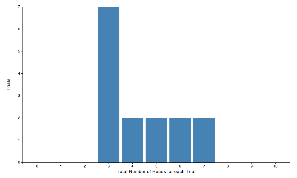
Looking at the results we see that the results are sort of centered around 5, but so far it looks like more outcomes are coming out lower than 5 than greater than 5. Let’s do 15 more trials and see if it looks any better.

Still looks like it leans to the left a bit. Lets do 30 more trials.

Finally, there are more 5’s. Let’s just go for gold and repeat the trial of ten flips 9,940 more times so we end up with a total 10,000 trials, each with 10 flips. This leads to the following plot.

The plot of the result of 10,000 trials of 10 flips looks pretty symmetric around 5, which is good. Looking at the plot you can make statements like if you flip a coin 10 times you are most likely going end up with 5H. Moreover, if you end up with 4H or 6H don’t freak out, those results are also pretty likely. Same with 3H and 7H. On the other hand, if you’ve flipped the coin 10 times and got only 2 or fewer heads or 8 or more heads, the particular result of your coin flips is not very likely to occur and the fact you observed it is a rarity.
Just for fun, we can try repeating the 10 coin flips another 90,000 more times to see if anything changes.

Meh… Looks pretty much the same. The shape really hasn’t changed at all. The same things are true as before. You’re likely to get 3, 4, 5, 6, or 7 heads, and you’re unlikely to get 0, 1, 2 or 8, 9, 10 heads. The only thing that is really different between the two plots is value recorded on the y-axis. If we look at the plot above, we see that roughly 2,400 of the 10,000 results of the 10 flips ended up producing 5 heads, whereas in this plot, roughly 24,000 of the 100,000 trials resulted in 5 heads. We postulate that if we did 1 million trials of 10 flips, we would expect roughly 240,000 trials to have resulted in 5 heads.
We can capture this idea by normalizing our plot so that height of the bar gives the probability of obtaining k heads in n=10 flips. Formally, this is called the binomial probability mass function and is given by the formula:

In our case the number of flips of each trial is n = 10, and since the coin is fair, the probability of obtaining a heads is p = 0.5. What we are after is the probability of obtaining a result, k. Let’s say we’re interested in the probability of flipping a coin 10 times and obtaining 5H. This means that we are looking for k = 5. Plugging into the formula tells us the probability is 0.2460938, or in other words, 24.61% of the time we should expect that result of 10 coin flips to produce 5 heads. Let’s plug in all the k’s from 0 through 10 and see what we get:
| Total Number of Heads for each Trial | Probability of Occurance |
| 0H | 0.0009766 |
| 1H | 0.0097656 |
| 2H | 0.0439453 |
| 3H | 0.1171875 |
| 4H | 0.2050781 |
| 5H | 0.2460938 |
| 6H | 0.2050781 |
| 7H | 0.1171875 |
| 8H | 0.0439453 |
| 9H | 0.0097656 |
| 10H | 0.0009766 |
And the plot of this looks like:

This plot is great because it gives us a visual representation of the likelihood of obtaining a certain number of heads if we flip a coin 10 times, given that we have a fair coin (equally likely to be heads as tails). The natural question, then, is what does it look like when our coin isn’t fair. Let’s say that we have a weighted coin so that 30% of the time it will land of heads and 70% of the time it lands on tails. The probability of obtaining a certain number of heads in 10 flips is given by the formula above with p = 0.3 and it looks like this:

The result is similar to the case of a fair coin, but the center of the distribution has moved to the left and the shape is skewed to the left a bit. Looking at the plot, we can say that getting 3 heads in 10 flips will occur most often, but we shouldn’t be too surprised if we get 1H, 2H, 4H, or 5H.
As another example, lets look at the plot for a weighted coin that lands on heads 60% of the time.

Same deal. The distribution is centered around 6H as expected, with 4H, 5H, 7H, and 8H being reasonably likely.
For our last example, lets look at the plot for a coin weighted to give heads only 10% of the time.

The skewing is pretty severe in this case since we’re butting up against left side of the plot (it is impossible to obtain fewer than 0 heads in 10 flips). The expected number of heads is 1 and likely results are 0H, 1H, 2H, and 3H.
So, to finally address this whole notion of statistical sampling uncertainty, let’s attack the problem the other way around. Let’s say we distribute mystery coins to 10 users on our site. The users are to flip the coins and if the coin lands on heads the user will click the “Add to Cart” button. If the coin lands on tails they leave the page. Although each of the coins is biased in the same way, the novel part of this scenario is that we don’t know how the coins are weighted. They could be a fair coins, or they all could be heavily biased toward heads or the coins could be all be biased towards tails. We just don’t know.
To reiterate our new scenario, we are going to flip 10 coins and measure how many heads we get. Each of the coins is biased in the same way, but we don’t know how they are biased. The goal of our experiment is to determine the bias of the coins.
We perform the experiment and flip 10 coins and obtain the following result:
T, H, T, H, H, T, T, T, H, T
There are 4H, or equivalently 4 our of 10 users clicked “Add to Cart”. What is the conversion rate?
A reasonable guess might be that the coin is biased to produce 40% heads and 60% tails. After all, getting 4 heads out of 10 is the most likely outcome for a coin biased that way. If the coin were biased 0.4 heads then using the binomial probability mass function we could compute the probability of our 4 heads measured outcome to be 0.251. On the other hand, what if the coin was biased at different way and we just happen to get 4H. If the coin were fair, then randomly getting 4H would have a probability of occurrence of 0.205, which still seems very reasonable. Likewise for a coin biased 30% toward heads you would obtain 4H with a probability of 0.200. Even if the coin were biased 60% towards heads, the probability of obtaining 4H is still greater than 0.11. And finally, if the coin were biased 20% heads, the probability of obtaining 4H is 0.088.
Lets tabulate some of the possible values of coin bias. In reality, the bias of the coin could be continually valued so in principle there should be many, many entries in the table, but for simplicity we’ll only tabulate half integer values.
| Assumed coin bais | Probability of 4H for assumed coin bias |
| 0.05 | 0.0009648 |
| 0.1 | 0.0111603 |
| 0.15 | 0.0400957 |
| 0.2 | 0.0880804 |
| 0.25 | 0.1459980 |
| 0.3 | 0.2001209 |
| 0.35 | 0.2376685 |
| 0.4 | 0.2508227 |
| 0.45 | 0.2383666 |
| 0.5 | 0.2050781 |
| 0.55 | 0.1595678 |
| 0.6 | 0.1114767 |
| 0.65 | 0.0689098 |
| 0.7 | 0.0367569 |
| 0.75 | 0.0162220 |
| 0.8 | 0.0055050 |
| 0.85 | 0.0012487 |
| 0.9 | 0.0001378 |
| 0.95 | 0.0000027 |
Let’s plot the table (normalizing so the total probability sums to 1) to see what it looks like

The plot looks roughly Gaussian but is is skewed slightly to the left. The distribution is actually Poissonian not Gaussian, but we need not concern ourselves with that subtlety right now. From inspecting the plot you can say that the best guess for the true bias of the coin is 0.4 and with 95% certainty the true bias of the coin will be between 0.2 and 0.65 heads. Not very satisfying is it. It is impossible to determine the bias of the coin to a high degree of accuracy by only looking at ten coin flips. We’ll see in a bit how to accurately report the confidence interval, but for now let’s try to find a way to lessen the sampling uncertainty.
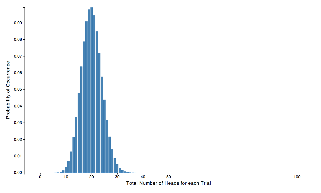
Since our analysis of 10 coin flips dead ended, what if we sample 100 visitors instead of 10. Well, we could repeat all of the steps we just did are reconstruct what the probability looks like for a fair coin (50-50) to land on heads k times in 100 flips, or we can skip right to the binomial probability mass function of the obtaining k heads with n=100 flips. It looks like this

We notice from this plot that is much narrower than Fig 6., meaning that the probable results are more concentrated in the middle. Looking at the numbers, it is reasonable to say that the expected value is 50 out of 100 heads, and we won’t be too surprised to get anywhere in the range 40 and 60 heads.
Just as a side note, the plot need not look so symmetric. If instead we had a coin that was biased 3% heads and 97% tails the probability mass function would look like this:

Now, just as we did before, lets turn the problem around and conduct an experiment where we measure the conversions of 100 visitors who have coins of unknown bias and try to guess the conversion rate (the bias of the coin).
We perform the experiment and the results are in. There were exactly 40 out of the 100 people who clicked the “Add to Cart” button. What’s our conversion rate?
Well a good guess would be 0.4 since the most probable result of a 0.4 biased coin would generate 40 successful conversions and that’s what we observed. However, reasoning along the same lines as before, wouldn’t a 0.2 biased coin be capable of producing 40 heads in 100 flips as well? Let’s plot a 0.2 biased coin and find out:
We can see from the plot that there is virtually no probability of obtaining exactly 40 heads with a 0.2 heads biased coin. The numerical value is only 0.0000023. While we were unable to rule out a 0.2 heads bias when we were only sampling only 10 users, after sampling 100 users we can now safely say that our coin does not have a 0.2 bias. The same goes for a coin with 0.6 bias towards head. The probability of obtaining exactly 40 heads for a 0.6 heads biased coin is only 0.0000244, so we can rule that one out as well. If you wanted to, you could tabulate a bunch of values like we did before to determine the 95% confidence interval. What you’d end up with is that the true bias of our coin is 0.4, with biases in the range 0.3 to 0.5 still being probable.
We’re on the right track. We’re much more confident about the bias of coin after taking 100 samples than we were after only taking 10 samples. The probability mass function is less wide for 100 compared to 10 samples which means that outcomes that far away from the mean are less probable.
Does this trend continue? What about for 1,000 samples? For a fair coin, the probability mass function looks like this:

The probability mass function is sharper still. Let’s do a similar sort of analysis as above. If we didn’t know the bias of our coin and we conducted an experiment where we obtained 400 heads our of 1,000 flips, we would be pretty sure that the true bias of our coin was 0.4 with a 95% confidence interval between 0.37 to 0.43. And if we did the whole thing again for 10,000 samples, and we obtained 4,000 heads in our experiment, then we would be pretty sure that the true bias of our coin was 0.4 with 95% confidence interval 0.39 to 0.41.
It should clear at this point that statistical sampling uncertainty can be mitigated by taking more data. Without taking sufficient data it is impossible to decrease this statistical sampling uncertainty. For example, if your intent is to make accurate statements about conversions rates within a few percent, it is imperative to take of order 1,000 measurements.
We feel that it is worth while to mention that not all results need to be known to super high accuracy. While it is difficult, it is not impossible to make fact based decisions with small sample sets. The pitfall you need to watch out for is statements like “Our users like our homepage. I called 10 people and 6 out of 10 say they like it a lot.” The conclusion that users like the the homepage is not supported by the facts. Saying “our users like our homepage” implies that more than half of the users like the homepage but having only sampled 10 people makes in very hard to make such a statement. On the other hand, one shouldn’t completely discount a 10 person sample. If none out of the 10 users like the homepage then it is likely that the majority of the users will not like the homepage. All data contains some information and your decision making abilities can be greatly enhanced by understanding how to properly interpret statistical results.
Back to the math. We mentioned earlier that its possible to produce some numeric values to better quantify the statistical sampling uncertainty. This is commonly quoted as a confidence interval. For sample sizes that are larger than 500 or so, as long as the conversion rate is greater than 1% (np > 5), the binomial distribution is roughly Gaussian and the central limit theorem applies. If this is the case, then the Wald approximation applies and the confidence interval is given by

In the equation, p is the average conversion rate of the sampled users, n is the number of samples taken, and z is the numeric value 1.96 in order to correspond to a 95% confidence level. If you have a good reason to prefer a different confidence level you can look up the corresponding value of z, but it’s standard practice to report 95% confidence so can just leave it at 1.96.
Sometimes it is too difficult or time consuming to collect 500 or more samples. Or, perhaps a particular funnel event has an extremely low conversion rate. In either of these cases the central limit theorem does not apply and you can’t use the Wald approximation. As a rule of thumb, you can’t use the Wald approximation when np < 5.
This was the case in the analysis of our original 10 coin flips. When we plotted the distribution of the possible true coin biases, the result was nearly Gaussian but not quite. The Wald interval assumes a Gaussian so it can’t be used in these extreme cases. We’ll need a different way to calculate the confidence interval.

This is the Wilson confidence interval, and meaning of the variables p, n, and z are the same as the were for the Wald approximation. The numerical values produced with the Wilson interval are more accurate than for the Wald interval for low conversion rates or small sample sizes, and nearly identical for middle of the road conversion rates or large sample sizes. As an illustration, an experiment with 100 samples and only 2 recorded conversions has a Wilson confidence interval of 0.038 ± 0.032. This means that we can say that the the true bias of the coin is 0.02 with 95% confidence that the true bias of the coin is between 0.006 and 0.07. Instead, if we had erroneously applied the Wald interval, we would get a confidence interval of 0.02 ± 0.027, which would lead us to say that the true bias of the coin is 0.02 with 95% confidence that the true bias of the coin is between 0 and 0.047, which is incorrect. In practice we tend to prefer the Wilson interval since it is more accurate and not too much more difficult to calculate.
Well that’s about all there is to it. Statistical sampling uncertainty naturally arises when looking at small sample sets. If you’ve collected some conversion data and want to know the conversion rate of a particular funnel event, you’re going to have to fight sampling uncertainty by taking enough data to make statements within your desired confidence interval. As a rule of thumb try to take 1000 samples (if it doesn’t take forever) and make sure that you’ve converted at least 5 people. In any case, if you report a the mean and Wilson confidence interval you’ll be accurately representing the data.
In the next blog post we’ll look at A/B testing and walk through the math needed to make statements like there’s a 90% chance that solution B is better than solution A.